Time series |
The most distinctive data type in Austra is the time series: a sorted collection of pairs date/value.
Since time series represents data from the real world, most of the times, time series come from persistent variables, that can be stored in an external file or database, and may be periodically updated, either by Austra or by another process.
Additional information in series
Since one of the goals of Austra is to deal with financial time series, there is a number of optional properties that can be stored in a series:
- Name
The name of the series is the name that is used by the parser to locate a series. For this reason, the series' name must be a valid identifier.
- Ticker
However, it's frequent for series to be identified by traders by their tickers, which is the name assigned by the provider of the series. A ticker is not necessarily a valid identifier, so we provide two different fields, one for the name and the second for a ticker. Tickers can be empty.
- Frequency
Each series has an associated frequency, which can be daily, weekly, biweekly, monthly, bimonthly, quarterly, semestral, yearly, or undefined. The library, at run time, checks that both operands in a binary operation have always the same frequency.
- SeriesType
In addition, each series has a type that can be either Raw, Rets, Logs, MixedRets, or Mixed.
Series versus vectors
Vector operations check, at run time, that the operands have the same length. The same behaviour would be hard to enforce for series. On one hand, each series can have a different first available date. On the other hand, even series with the same frequency could have reported values at different days of the week or the month, and still, it could be interesting to mix them.
So, the rules for mixing two series in an operation are:
They must have the same frequency, and their frequencies are checked at runtime.
However, they may have different lengths. If this is the case, the shorter length is chosen for the result.
The points of the series are aligned according to their most recent points.
The list of dates assigned to the result series is chosen arbitrarily from the first operand.
Class methods
There is only one constructor for series:
series::new | Creates a linear combination of series. See Combine. |
The first parameter of series::new must be a vector of weights, and from that point on, a list of series must be included. This class method creates a linear combination of series. The length of the weights vector can be equal to the number of series or the number of series plus one. For instance:
series([0.1, 0.9 ], aapl, msft);-- The above code is equivalent to this:
0.1 * aapl + 0.9 * msft
If we add another item to the vector, it will act as an independent term:
series([0.5, 0.1, 0.9 ], aapl, msft);-- The above code is equivalent to this:
0.5 + 0.1 * aapl + 0.9 * msft
We can also import a series from any CSV file that has a date and a double-valued column:
let curves = csv("curves.csv" ) .withHeader.withSeparator("," ).withFormat("EN-US" );-- You can use both column names and column indexes. series("SONIA" , curves.withFilter("Curve Name" ,"SONIA" ),11, 15 ); series("SONIA" , curves.withFilter("Curve Name" ,"SONIA" ),"Curve Maturity Date" ,"Zero Rate Curve value" );
Series properties
These properties are applied to instances of series:
acf | The AutoCorrelation Function. See ACF. |
amax | Gets the maximum of the absolute values. See AbsMax. |
amin | Gets the minimum of the absolute values. See AbsMin. |
count | Gets the number of values in the series. See Count. |
fft | Gets the Fast Fourier Transform of the values. See Fft. |
first | Gets the first point in the series (the oldest one). See First. |
fit | Gets a vector with two coefficients for a linear fit. See Fit. |
kurt | Get the kurtosis. See Kurtosis. |
kurtp | Get the kurtosis of the population. See PopulationKurtosis. |
last | Gets the last point in the series (the newest one). See Last. |
linearFit | Gets a line fitting the original series. See LinearFit. |
logs | Gets the logarithmic returns. See AsLogReturns. |
max | Get the maximum value from the series. See Maximum. |
mean | Gets the average of the values. See Mean. |
min | Get the minimum value from the series. See Minimum. |
movingRet | Gets the moving monthly/yearly return. See MovingRet. |
ncdf | Gets the percentile of the last value. See NCdf. |
pacf | The Partial AutoCorrelation Function. See PACF. |
perc | Gets the percentiles of the series. See Percentiles. |
random | Creates a random series from a normal distribution. See Random. |
rets | Gets the linear returns. See AsReturns. |
skew | Gets the skewness. See Skewness. |
skewp | Gets the skewness of the population. See PopulationSkewness. |
stats | Gets all statistics in one call. See Stats. |
std | Gets the standard deviation. See StandardDeviation. |
stdp | Gets the standard deviation of the population. See PopulationStandardDeviation. |
sum | Gets the sum of all values. See Sum. |
type | Gets the type of the series. See Type. |
var | Gets the variance. See Variance. |
varp | Gets the variance of the population. See PopulationVariance. |
values | Gets the underlying vector of values. See Values. |
Series methods
These are the methods supported by time series:
all | Checks if all items satisfy a lambda predicate. See All. |
any | Checks if exists an item satisfying a lambda predicate. See Any. |
ar | Calculates the autoregression coefficients for a given order. See AutoRegression. |
arModel | Creates a full AR(p) model. See ARModel. |
autocorr | Gets the autocorrelation given a lag. See AutoCorrelation. |
corr | Gets the correlation with a series given as a parameter. See Correlation. |
correlogram | Gets all autocorrelations up to a given lag. See Correlogram. |
cov | Gets the covariance with another given series. See Covariance. |
ewma | Calculates an Exponentially Weighted Moving Average. See EWMA. |
filter | Filters points by values or dates. See Filter. |
indexOf | Returns the index where a value is stored. See IndexOf. |
linear | Gets the regression coefficients given a list of series. See LinearModel. |
linearModel | Creates a full linear model given a list of series. See FullLinearModel. |
ma | Calculates the moving average coefficients for a given order. See MovingAverage. |
maModel | Creates a full MA(q) model. See MAModel. |
map | Pointwise transformation of the series with a lambda. See Map. |
movingAvg | Calculates a Simple Moving Average. See MovingAvg. |
movingNcdf | Calculates a Moving Normal Percentile. See MovingNcdf. |
movingStd | Calculates a Moving Standard Deviation. See MovingStd. |
ncdf | Gets the normal percentil for a given value. See NCdf. |
stats | Gets monthly statistics for a given date. See GetSliceStats. |
zip | Combines two series using a lambda function. See Zip. |
Operators
These operators can be used with time series:
+ | Adds two series, or a series and a scalar. |
- | Subtracts two series, or a series and a scalar. Also works as the unary negation. |
* | Multiplies a series and a scalar for scaling values. |
/ | Divides a series by a scalar. |
.* | Pointwise series multiplication. |
./ | Pointwise series division. |
Points in a series can be access using an index expression between brackets:
aapl[0 ]; aapl[appl.count -1 ].value = aapl.last.value; aapl[^2] = aapl[aapl.count - 2 ]
Series also supports extracting a slice using dates or indexes. In the first case, you must provide two dates inside brackets, separated by a range operator (..), and one of the bounds can be omitted:
aapl[jan20..jan21]; aapl[jan20..15 @jan21]; aapl[jan20..]; aapl[..jan21]
The upper bound is excluded from the result, as usual. Date arguments in a series index do not support the caret (^) operator for relative indexes. When using numerical indexes in a slice, the behaviour is similar to the one of vectors:
aapl[1..aapl.count - 1].count = aapl[1..^1].count
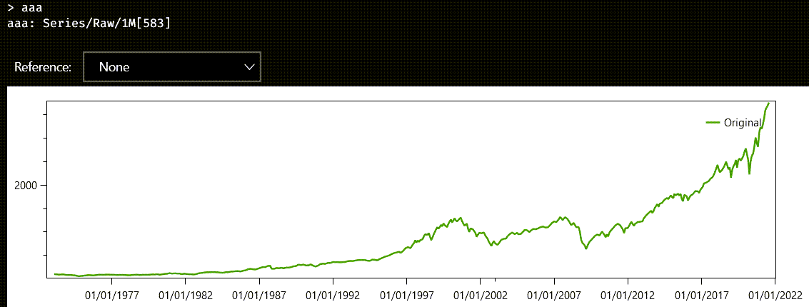
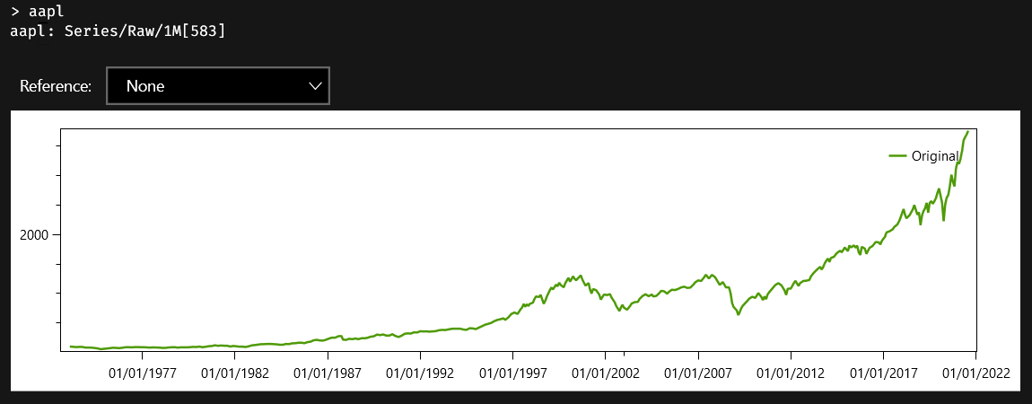
When you face a time series for the first time, the first thing you want is to decompose the series in all its identifiable components. The series may be the sum of a linear or quadratic process, it may have seasonal variations or any kind of period-ic variation, it may show signs of a stochastic process such as an autoregressive or moving average process and there will be almost always a random noise in the raw data.
The most easily identifiable component is perhaps a linear trend in the data. Look at the chart of this raw series with monthly sampling:
If you apply the fit method to this series, the answer will be two numbers in a real vector:
aaa.fit-- This is the answer:
ans ∊ ℝ(2)
0.134716 -97404.4
The first number in the vector is the slope, and the second number is the intercept, that is, the value when the argument of the corresponding line is zero. If you wanted to look at the inferred line, you could execute the linearFit property on aaa, which creates a series with the same date, but with values from the fitted line. You can also subtract aaa.linearFit from aaa, to see the part of the data that cannot be explained by a simple line model:
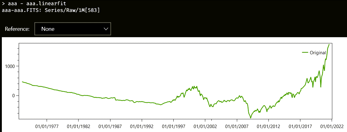
Austra uses Ordinary Least Squares (OLS) to find the coefficients of the fitting line.
If your data cannot be easily explained using a simple line, you could try another approach: explaining a series as a linear combination of other existing series. Let us say that we want to explain the aaa series using three other series. This is the formula we need:
aaa.linearModel(aab, aac, aad)
An instance of the LinearModel class is created, and this is how the Austra Desktop application shows it:
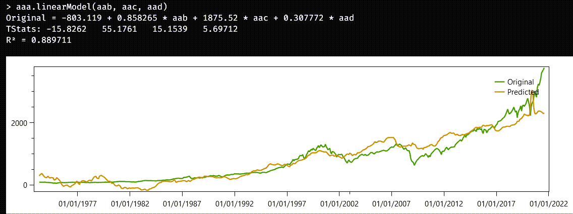
The most important data is contained in the first line of the answer:
aaa=-803.12+0.858*aab+1875.52*aac+0.308*aad
That is how the series to be explained can be approximated with the other three predicting series. Coefficients are calculated to minimize the OLS of the difference between the prediction and the original.
The second line give us the t-statistics for the relevance of each coefficient. Note, for example, that the most relevant coefficient is the one corresponding to the aab series, even though the coefficient for aac is greater. The reason is that values from aac are smaller than values from aab. The next line gives us the R2 statistics, also known as goodness of fit, which is the quotient between the explained variance and total variance. The closer R2 is to one, the better the explanation is.
Finally, the application shows a chart including the original and the predicted series.
In case you only need the coefficients of the model, you can call the linear method on aaa, using the same parameters as before. linear just returns a vector with the coefficients used in the model.
A fair share of the properties and methods implemented by series has to do with statistics, either of the whole series or of partial samples from the series. Most of these properties and methods are shared with real vectors and sequences, for obvious reasons.
The next few sections deal with time series features that computes statistics for a time series.
Accumulators
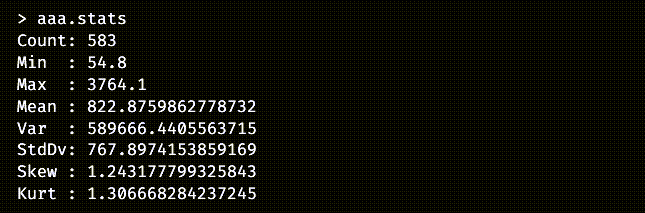
The stats property returns an object from the C#’s Accumulator class that holds statistics on all samples from the series.
The Accumulator class defined by the Austra library, implements a running accumulator that calculates and updates the most important statistics estimators as we keep adding values from a dataset, using the well-known Welford algorithm. Our implementation of Welford’s algorithm takes advantage of SIMD instructions from the CPU, when available. Since it is a fast implementation, the result returned by the stat property from a series is always computed when the time series is created. Persistent series are created when the Austra Desktop application starts up, or when a series is retrieved the first time from an external service or database. This way, you can always call stats without concerns about efficiency, and the same is valid on any property derived from the running accumulator.
Most of the properties of stats are also available as direct properties of the series, for convenience. They are:
count | Gets the number of values in the series. See Count. |
kurt | Get the kurtosis. See Kurtosis. |
kurtp | Get the kurtosis of the population. See PopulationKurtosis. |
max | Get the maximum value from the series. See Maximum. |
mean | Gets the average of the values. See Mean. |
min | Get the minimum value from the series. See Minimum. |
skew | Gets the skewness. See Skewness. |
skewp | Gets the skewness of the population. See PopulationSkewness. |
std | Gets the standard deviation. See StandardDeviation. |
stdp | Gets the standard deviation of the population. See PopulationStandardDeviation. |
var | Gets the variance. See Variance. |
varp | Gets the variance of the population. See PopulationVariance. |
Remember that most of all these properties are just estimators, and that their accuracy depends on the number of samples. Skewness and kurtosis, for example, needs more than a thousand samples for an approximate ballpark estimation, at least, according to my own experience.
One nice property about running accumulators is that you can combine two of them easily and efficiently using the plus operator:
aaa.stats + aab.stats
A stats property is also implemented by real and integer vectors and sequences.
Moving time windows
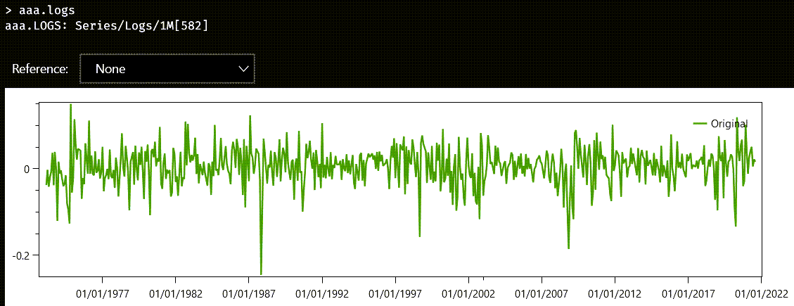
A series like our friend aaa is classified as a raw series. It starts with low values, and, despite random oscillations, it has a definite upward trend. If we take the mean of the first half of the series, it will be wildly different from the other half’s mean. The average value is not a significant property of the series.
Part of the problem has to do with the fact that aaa probably represents a random walk. The most probable underlying process that generates a series like this works by throwing a die at each step and deciding how much we must increase or decrease the current value. We can focus, however, on how these variations behave, by transforming the series into a series of returns. Series have two properties for this task: rets, for linear or ordinary returns, and logs, for logarithmic returns. This chart shows the logarithmic returns of aaa:
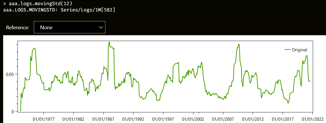
Now we have a series with a uniform mean throughout its lifetime, but another problem has surfaced. The time range we sample has a significant impact on the variation in the returns. In other words, different segments have different standard deviations or variances.
That is the reason why there are series methods like movingAvg, movingStd, and movingNcdf that calculate those statistics over a sliding window of samples. Each of these methods requires the number of samples to define the moving window. Since aaa is a monthly series, the following chart displays the accumulated standard deviation for a moving period extending from one year.
The related property, movingRet, can be used on raw and return series and averages the return according to the sampling frequency of the series. In this case, we do not supply the size of the sliding window, but it is inferred from its type and frequency.
Autocorrelation and partial autocorrelation
There are two important diagnostic functions on series: the autocorrelation function, also known by the acronym ACF, and the partial autocorrelation function, also known as PACF.
The ACF is defined as the Pearson correlation between a signal and a delayed copy of the signal. The argument of the function is the delay between the samples and, since we are dealing with discrete signals, the type of the argument is an integer value.
There are formulas that work better with stationary series, that is, series with uniform statistical properties, widely speaking. Most financial series are not stationary, when the sampling time is long enough, as we will see soon. Our algorithm does not assume stationarity and is based on the Wiener-Khinchin theorem, that relates the autocorrelation function with the power spectral density via the Fourier Transform. Internally, Austra calculates a Fast Fourier Transform on a padded version of the series, using the next available power of two size for speed.
The Partial Autocorrelation Function, or PACF, is closely related but must not be confused with the ACF. The PACF measures the direct correlation between two lags, without accounting for the transitive effect of any intermediate lags. Our PACF implementation calculates the ACF as a prerequisite, and then performs the Levinson-Durbin algorithm on the ACF to remove those spurious effects from the lags in-between.
Autoregressive models
The autoregressive model is one of the simplest stochastic models that can generate a time series. If we denote as x(t) the value of a series at a time or step t, an autoregressive model of order p is a process generated by this formula:
The ε(t) term is a random value taken from any distribution, not necessarily a standard one. It is only required that the mean of ε(t) be zero. If the order of the model, p, is zero, what remains is just white noise. And things start getting interesting when p>0, because each term start been influenced by a subset of the preceding terms in the series.
The easiest way to generate an autoregressive model for testing is using class methods from real sequences. What series provide are methods for estimating parameters for an autoregressive model, assuming that the series has been generated by such a model. The arModel method estimates coefficients and includes some useful statistics with the output. The ar method is a leaner version of arModel that only returns coefficients. Finally, you can use the pacf property to check if an autoregressive process would be a good guess about how the series has been generated.
Let us take as example our good-old aaa series:
This is not a stationary series, and it looks more like a random walk. But an autoregressive process can yield random walks instead of stationary series when the sum of the coefficients is high enough. We will start by calculating the Partial Autocorrelation Function of the samples we have. Theory says that partial autocorrelations for an autoregressive model falls to zero after a few lags. And that is just what we see when we plot the full PACF of aaa:
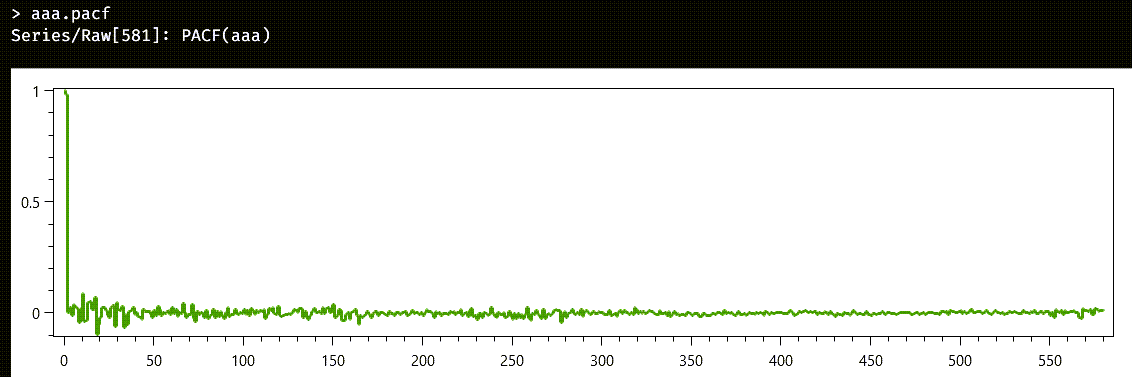
The return type of properties like acf and pacf is series<int>: instead of the usual pairs containing date/value, here we return pairs containing lag/value. Unfortunately, the control used for the chart does not have all the whistles and bells we would want. So, lets manually zoom on the first lags, to see what is happening.
Since series stores their values in reverse order, what we really want is a slice from the end of a series, so we will evaluate this formula:
aaa.pacf[^20..^0 ]
And this is the new chart we get:
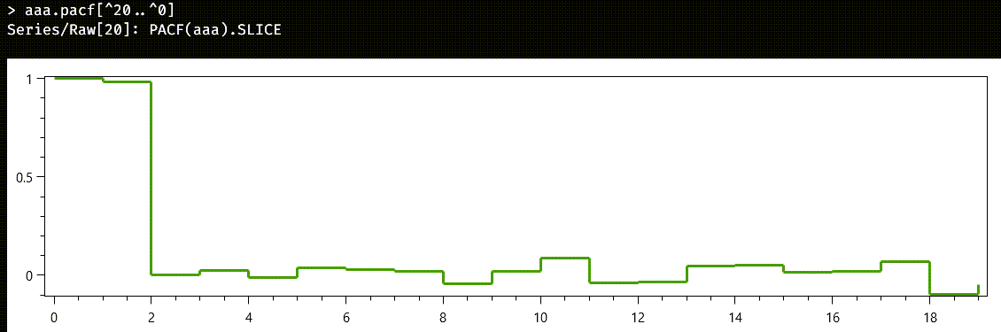
The first value of both the ACF and the PACF functions corresponds always to the lag zero, so it is always one. The value for the lag one is near one, and then, all the rest of the partial autocorrelations are negligible. We will bet that we can model the series with an autoregressive model of degree 1, and we are pretty sure that the coefficient will be high enough to generate a random walk instead of a stationary series. We will use the more nuanced method arModel to get as information as possible:
aaa.arModel(1 )
And voilà, here we have the estimated model:
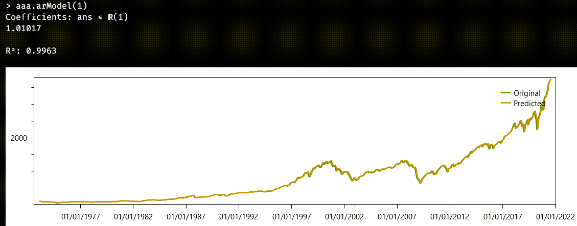
As we already suspected, the coefficient is greater than unity. The r2 property of the model is the same goodness of fit we have already seen with linear models. It is the quotient of the explained variance over the total variance, and it is high enough for the model to be considered a good one.
The chart plots both the original series and the “predicted” one. As a word of caution, don’t be fooled by the word “prediction”: what we are forecasting is just one step forward, assuming the historically attested levels. It would be impossible, as it stands to reason, to generate the whole series from an initial level and the autoregressive law.
Austra estimates coefficients for AR models using the so-called Yule-Walker equations. |
Moving Average models
Another common process that generates a time series is the algorithm known as Moving Average. A Moving Average process of order q, often referred as MA(q), is defined by the following formula:
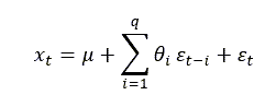
This is a very different beast that the autoregressive models we have already seen. All the ε(i) terms still refer to random variables centred around zero. We also have a new term, μ, which is interpreted as the mean of the series. What makes different an MA model from an AR one is that what is propagated to successive steps is not the actual value at a past time, but the error term introduced in a previous step.
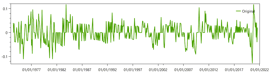
Pure Moving Average series are stationary series. Since I do not have a good real candidate at hand, I will use a transformed series as the source of the MA example. I have an aac series, and I will take its linear returns as my original samples. Even then, the resulting series is not a stationary one, so the match will not be perfect. This is how I get the linear returns from a time series:
aac.rets
And this is the corresponding chart:
For MA series, we must use the ACF instead of the PACF. These are the fifty first lags of the ACF:
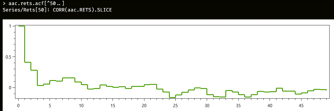
This time, the cutoff is not as clear as before. Let us start by trying an MA(2) model:
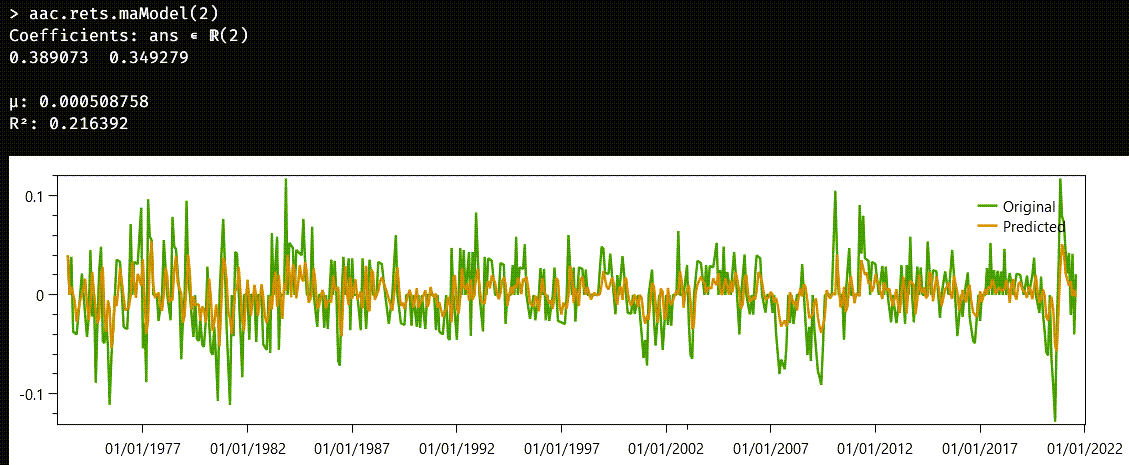
It could have been worse. The r2 statistics is nothing to write home about. Note that, this time, we also have the μ parameter for the mean of the series. We could keep rising the number of the degrees of the model for a better match, but we would soon meet diminished returns. Remember that the original series was not a stationary one.
MA models are way harder to estimate than the simpler AR model. The depend on past “errors”, which are not directly observable, but must be inferred from the samples. |