Vectors

AUSTRA provides double-precision vectors, identified by the class vec, complex double-precision vectors, cvec, and vectors of integer, ivec. All these data types are implemented using dense storage.

A vector is constructed by listing its components inside brackets:

[1, 2, 3, 4]

Commas are mandatory for separating items, and white space and line feeds are always ignored.

Bracket lists can be also used to concatenate the content of several vectors, and you can add scalars to the mix:

let v1=[1, 2], v2=[3, 4];
-- Returns a vector with 4 items.
[v1, v2];
-- This also is accepted:
[[1, 2], v2];
-- Scalars can also be added.
[0, v1, pi, v2, tau];

Class methods

Vectors can also be created using these class methods:

These are the overloads supported by vec::new:

-- Creates a vector with 10 items, all of them zeros.
vec::new(10);
-- Remember that ::new can be omitted!
vec(10);
-- Creates a vector like [1 2 3 4 5 6 7 8 9 10]
vec(10, i => i + 1)

The last example shows how to create a vector using a lambda function parameter. This is a more sophisticated example of using a lambda to initialize items in a vector:

-- Mimics a periodic function.
vec(1024, i => sin(i*pi/512) + 0.8*cos(i*pi/256))

vec::new can also be used to create a linear combination of vectors:

vec([0.5, 0.1, 0.7, 0.2], v1, v2, v3)

The first parameter contains weights, and the remaining parameters are the vectors that will be linearly combined. If there is an extra value in the weights, as in the example, it is used as an independent term. The above expression is equivalent to this one:

0.5 + 0.1 * v1 + 0.7 * v2 + 0.2 * v3

Please note that the parser can detect some code patterns and optimize expressions automatically. For instance, for vectors, the parser recognizes these patterns:

vector1 * scalar + vector2;
scalar * vector1 + vector2;
scalar1 * vector1 + scalar2 * vector2;

All these expressions are reduced to calls to one of the overloads of either MultiplyAdd or Combine2. These methods are internally optimized to use a single temporary buffer, instead of the two buffers of a naïve implementation, and both of them use FMA fused operations when available. Of course, the method underlying the above presented vec::new constructor is even better optimized and runs several times faster than even the optimized versions of lineal composition.

Another experimental optimisation substitutes non-destructive operators by operations that directly modify the internal buffer of one of the operands:

vec::random(10) + vector2;

It does not matter where vector2 comes from. The first operand is a "new" vector, created on the fly for this formula, and its buffer will not survive beyond this formula. The compiler reckons it is safe to substitute the non-destructive addition with a version that leaves the result in the buffer of the first operand.

Vector properties

Properties and methods or vectors are very similar to the ones from series. As a rule, almost all code in series that do not need to take dates into account, is implemented via the corresponding vector code, which is heavily optimized and hardware-accelerated. These are the properties supported by a vector instance:

Vector methods

These are the methods supported by a vector instance:

Vector operators

Real-valued vectors supports the basic repertoire of operators:

The outer product of vectors x[i] and y[i] returns the matrix with components m[i,j]=x[i]*y[j]. This expression call:

[1,2,3]^[4,5,6]

returns this matrix:

ans ∊ ℝ(3⨯3)
 4   5   6
 8  10  12
12  15  18

There's no special syntax for complex vector literals, but complex vectors can be easily created using the cvec::new class method and one or two vector constructors:

cvec::new([1, 2, 3, 4], [4, 3, 2, 1]);
-- ::new can be omitted.
cvec([1, 2, 3, 4], [4, 3, 2, 1])

These class methods are available for creating complex vectors:

These are the overloads supported by cvec::new:

-- Creates a complex vector with 10 zeros.
cvec(10);
-- Creates a complex vector from one real vector.
cvec([1, 2, 3]);
-- Creates a complex vector from two real vectors.
cvec([1, 2, 3], [3, 2, 1]);
-- Creates a complex vector with a lambda function.
cvec(10, i => polar(2π*i/10));
-- The lambda function includes access to the complex vector.
cvec(100, (i, v) => polar(2π*i/10) - 0.01 * i * v{i-1})

Complex vector properties

These are the properties supported by a complex vector instance:

Complex vector methods

These are the methods supported by a complex vector instance:

Complex vector operators

Complex vectors supports the same operators as real-valued operators, with the exception of the outer product ^. On the other hand, they add support for complex vector conjugation using a unary suffix operator:

Complex vector conjugation inverts the sign of each imaginary component in the vector. The inner product of two complex vectors actually conjugates the second vector operand.

Integer vectors are also supported, using the ivec class.

ivec::random has three overloaded variants:

-- Ten items. Values between 0 and int.MaxValue - 1.
ivec::random(10);
-- Values between 0 and 999.
ivec::random(10, 1000);
-- Values between -10 and 9.
ivec::random(-10, 10)

Integer vector literals can be created using this notation:

-- Integer vector creation.
let v1 = [int: 1, 2, 3, 4];
-- Integer vector concatenation.
[int: v1, 5, v1.reverse];

Integer vector properties

Integer vectors support these properties:

Integer vector methods

These are the methods for integer vectors:

Individual values from vectors are accessed using its position, starting from zero, inside brackets:

vec[0];
vec[vec.length - 1]

A segment or slice can be extracted as another vector by using this notation:

vec[1..vec.length - 1]

The above expression removes the first and the last element from a vector. The upper bound is excluded.

The caret (^) can be used in indexes and segments, to count positions from the end. For instance, this expression returns the next to last item of a vector:

vec[^1]

These equalities hold:

vec[1..^1] = vec[1..vec.length - 1];
vec[^5..^2].length = 3

Vectors and series also support safe indexers. With normal indexers, like v[1000], an out-of-range reference throws an exception and interrupts the evaluation of the formula. If braces are used instead of brackets, and out-of-range reference returns 0.0 and it is considered as a valid use. For instance, the following expression returns zero:

[1, 2, 3, 4]{1000}

Safe indexers are useful when used inside lambda functions. This expression creates a vector holding the first 30 Fibonacci numbers:

vec(30, (i, v) => max(1, v{i-1} + v{i-2}))

AUSTRA provides a Discrete Fourier Transform for real and complex vectors, sequences, and series. The core result of the transformation, which is implemented by the fft property is a complex vector, but this vector is commonly wrapped inside a FftModel class instance, which provides additional helping methods and properties and, among them, a method for inverting the transform and getting back the original samples.

The other function of FftModel is to act a semantic marker on behalf of any application that is using the AUSTRA parser. When you execute something like aaa.fft in the Austra Desktop application, where aaa is a time series, you get a special view for the Fast Fourier Transform based on the returned FftModel:

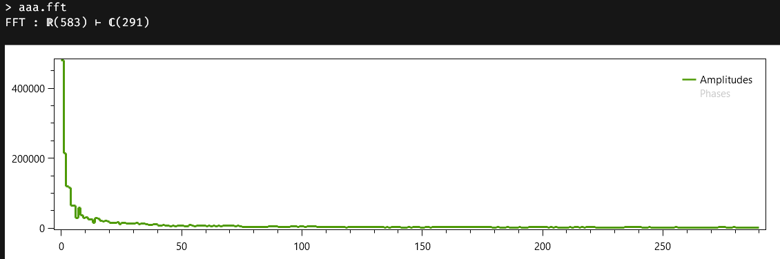
The first line tells us we are seeing a Fast Fourier Transform that has transformed 583 real samples into a complex spectrum containing 291 complex values. Since there is not a pretty and effective way to draw those complex values, the chart that follows shows the amplitudes of those values, and gives us the option to also see their phases.

If we immediately type and execute ans.inverse, we would get not the original series, because the date arguments has been discarded by the FFT, but a vector with the original values or coordinates of the time series. The key in the recon-struction is that the FftModel keeps track of the fact that the FFT was created from a vector of reals instead of from a vector of complex numbers.

Let us check now how our FFT handles a complex vector. For making things a little more interesting this time, we are going to start with this formula:

(cvec::nrandom(1024) + cvec(1024, i => 0.6*sin(i*0.2))).fft

There is a noisy component, based on a normal distribution, and then we add a shameless periodic function, affecting just the real part of the complex vector. The first thing we can predict is that the FFT will not have a big zero component: the zero component of any Discrete Fourier Transform is known as the DC, or Direct Current component, in electronic jargon, because it represents the mean of the samples. Our new mean will be insignificant, because the normal distribution generates both positive and negative terms, and the corresponding plot confirms our suspicions:

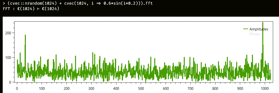
This time, the number of samples in the transform is the same number of original samples. It is immediately obvious that there is a periodic component in the samples, which shows as two symmetric peaks at the beginning and end of the spectrum. And, if we immediately execute ans.inverse, we get back the original complex vector, with all its samples.

FFT properties and indexer

For the sake of clarity, let us group all properties available for FFT models:

The FftModel class also implements an indexer and allows the use of slices and relative indexes.

Reference

Other Resources