Models

The model class is a general-purpose container for algorithms that do not fit well as members of other classes. These models are generally shown by the Austra Desktop application as interactive controls, allowing users to explore the whole range of solutions available for each model.

Mean variance optimisation (MVO) is a mathematical optimisation for maximising the expected return of a portfolio given a level of risk. Inside a polytope, the fundamental algorithm is an optimizer for a quadratic objective function. A polytope is just a fancy name for a polyhedron in a high-dimensional space.

The MVO is implemented by the MvoModel class from the Austra library, and it is available for the AUSTRA language by executing the model::mvo class method.

Let us assume we have a portfolio with three assets, and we want to find the three optimal weights, one for each asset. The most general method overload of the MVO would be like this:

-- This example assumes we are dealing with three assets.
model::mvo(
    -- A 3D-vector for returns and a 3x3 covariance matrix.
    retVec, covMatrix,
    -- Two 3D-vectors for lower and upper bounds.
    [0, 0, 0], [1, 1, 1],
    -- A label for easy identification of each asset.
    "Name1",
    "Name2",
    "Name3")

• We have purposefully avoided stating any values for the retVec and covMatrix variables. These two variables would contain a vector with the expected return of each asset and a covariance matrix for these assets.
• It is not obvious how expected returns are to be calculated. Financial series are seldom stationary, so the expected return would normally depend on time.
• The covariance matrix faces a similar problem.
• The lower and upper bounds, on the contrary, are generally easier to set; they are just the minimum and maximum weights we desire for each asset in the portfolio.
• The MVO algorithm automatically adds another condition for the weights: their sum must be equal to one.

For the sake of the example, we are going to assume an arbitrary rentability for each of our three hypothetical assets. For the covariance matrix, we will make things more interesting by creating a fake matrix with three of our series examples: aaa, aab and aad:

> matrix::cov(aaa, aab, aad)
ans ∊ ℝ(3⨯3)
 589666   525180  19023.8
 525180   553027  16232.4
19023.8  16232.4  42045.1

The main diagonal of the above matrix tells us how volatile each of our assets is. We can see that aaa has the greater variance and that aad has the lesser variance and, consequently, the lower associated risk. So, we will assume that the first asset provides the better return, followed by the second and third assets:

model::mvo(
    [1, 0.8, 0.6],
    matrix::cov(aaa, aab, aac),
    [0, 0, 0], [1, 1, 1],
    "Name1", "Name2", "Name3")

If we execute this code, we will get the following interactive output in the area with results from the Austra Desktop application:

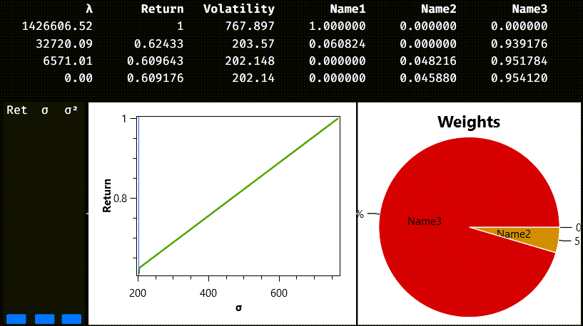
The first part of the output is a table enumerating portfolios from the so-called efficient frontier. There are four such portfolios in our example. The first portfolio maximises the expected return, but it is also the one with more volatility, or risk. This portfolio only includes the first asset; the weight for this asset is one, and the rest of the weights are zero. The last listed portfolio is the one with the lesser vola-tility and return, and it is a mix of the second and third assets. Each portfolio in-cludes a value for the lambda column, which mathematically is the value of the Lagrange multiplier for this solution. From the business point of view, lambda is an indicator of the associated risk.

Portfolios in the efficient frontier are important because they represent turning points in the strategy for changing asset weights. Any portfolio interpolated from two portfolios on the efficient frontier is a viable solution to our problem. And that is the mission of the three sliders on the left side of the charts: you can select ei-ther a desired return, a standard deviation, or a variance, and the charts will show you which weights are needed for the selected portfolio. This is what we get if we choose an expected return of approximately 0.8:

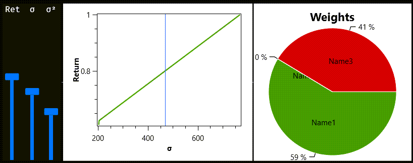
The required portfolio must be a combination of 59% from the first asset and another 41% from the third asset.

More class method overloads

For our example, we chose arbitrary names for the assets that compose our portfolio. When these assets are related to series in our session, it is easier to use the name of the series for this task:

model::mvo(
    [1, 0.8, 0.6],
    matrix::cov(aaa, aab, aac),
    [0, 0, 0], [1, 1, 1],
    aaa, aab, aad)

Now, the series variables are mentioned twice in the formula. We could change the formula this way:

model::mvo(
    [1, 0.8, 0.6],
    aaa, aab, aad)

This is the simplest method overload for the MVO. Note that we have also removed the lower and upper bounds, making the natural assumption that all weights will stay in the [0,1] interval. We still need, however, to explicitly state the expected returns, but Austra infers that we want to use the covariance matrix for the three used series.

Additional constraints

Optimization problems frequently include additional constraints beyond the simple limits we have shown so far. As a matter of fact, since we have not included a constraint for the total sum of weights, the model::mvo method has automatically added this constraint to the problem:

Let’s say we want another constraint. For instance, the first asset’s weight must always be greater or equal to the third asset's weight:

The most general form for this kind of constraint is a list of equations following this pattern:

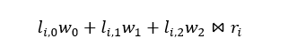
Here, l stands for left side and r means right side. That strange symbol ⋈ only means that we can substitute it either with an equality or an inequality. So, more generally, our additional constraints could always be written as:

L is a matrix with as many columns as assets in the problem and an arbitrary number of rows, r is a vector with the same number of items as rows in the left-side matrix. Still, we must find a way to determine which relational operator must be used for each of the constraints.

The MvoModel class provides an overloaded method for adding constraints to an already existing model:

mvoModel.setConstraints(lhsMatrix, rhsVector, opsIntVector)

The first parameter must be a matrix; the second parameter must be a real vector; and the third parameter must be an integer vector. Items in the third parameter are interpreted according to their signs. A positive value means a greater or equal operation; a negative value stands for a lesser or equal relationship; and zero means equality. The third parameter can be omitted when all constraints are equality constraints.

This way, if we want to combine the sum-of-weights constraint with our additional constraint, we will need the following code:

model::mvo(
    [1, 0.8, 0.6],
    aaa, aab, aad).setConstraints(
        [1, 1, 1; 1, 0, -1], [1, 0], [int:0, 1])

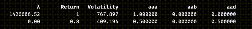
These are the portfolios from the efficient frontier, with the additional constraint:

We could even drop the first constraint because the optimiser will add it when it is not present:

model::mvo(
    [1, 0.8, 0.6],
    aaa, aab, aad).setConstraints(
        [1; 0; -1]’, [0], [int:1])

Please note the trick we need to create a matrix literal with only one row; we wrote it as a one-column matrix and then transposed it. This is a valid alternative:

model::mvo(
    [1, 0.8, 0.6],
    aaa, aab, aad).setConstraints(
        matrix::rows([1, 0, -1]), [0], [int:1])

The model class also provides a simplex method for solving linear programming problems. In a typical linear programming problem, we must maximize the value of a linear function like this:

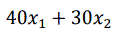
All variables are implicitly considered non-negative, and some additional constraints must be satisfied:

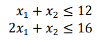
This problem can be solved using this code:

model::simplex([40, 30], [1, 1; 2, 1], [12, 16], [int: -1, -1])

The first parameter contains the coefficients from the objective function. The second parameter is a matrix with the left-hand side coefficients of the constraints, and the third parameter is the right-hand side of the constraint as a vector. Finally, the last parameter contains the relational operators for each constraint. Since all constraints have the same sign, we can simplify the code like this:

model::simplex([40, 30], [1, 1; 2, 1], [12, 16], -1)

In both cases, the answer is a SimplexModel object that contains the optimal value and the coefficients for the optimal solution:

> model::simplex([40, 30], [1, 1; 2, 1], [12, 16], [int: -1, -1])
LP Model (2 variables)
Value: 400
Weights:
  4    8

This method always assumes that we want to maximize the value of the objective function. If you want to minimize the objective function, you could invert the sign of the coefficients:

model::simplex(-[12, 16], [1, 2; 1, 1], [40, 30], +1)

Note, however, that doing by this, you will get a negated value for the solution.

LP Model (2 variables)
Value: -400
Weights:
 20   10

You can fix this problem by using simplexMin instead and using the original coefficients in the objective function:

model::simplexMin([12, 16], [1, 2; 1, 1], [40, 30], +1)

Other Resources